Ways to Decompose a Face

Introduction

Eigenfaces are a cool application of SVD. Feed a bunch of face photos into it and you get back a set of “average” faces that can be mixed together to rebuild any face in the dataset. We’ll build them from scratch, then look at a second approach (NNMF) that pulls out localized features like eyes and noses instead of full-face blends.

SVD

SVD, or Singular Value Decomposition, is a way of breaking any matrix down into three simpler pieces that reveal its underlying structure.

But what does this mean?

Let’s say we have a matrix $M \in \mathbb{R}^{m \times n}$. We can write it as $M = U \Sigma V^T$, where $U \in \mathbb{R}^{m\times m}$ and $V \in \mathbb{R}^{n \times n}$ are orthogonal matrices, and $\Sigma \in \mathbb{R}^{m \times n}$ is a diagonal matrix whose entries $\sigma_1 \geq \dotsb \geq \sigma_r > 0$ are the singular values. Visually, $\Sigma$ looks something like this, where the empty spots are just zeros:

Intuitively, each piece has its own job:

1. $V^T$: rotates the data into a new coordinate system aligned with its most important directions
2. $\Sigma$: scales each direction by how much variance it captures
3. $U$: expresses each original data point as a combination of those directions

The nice thing is this works for any real matrix $M$. Since the singular values are sorted from big to small, the most important structure in the data lives in the first few $\sigma_i$. Keep just the top $r$ of them and you get the best rank-$r$ approximation of $M$.

Coding

Loading the Data

Let’s apply this. First we’ll load a dataset and reshape it into something we can feed to SVD. This is mostly boilerplate, so feel free to copy it.

import kagglehub
import numpy as np
import os
import cv2
import matplotlib.pyplot as plt

path = kagglehub.dataset_download("jessicali9530/celeba-dataset")

def load_images(image_directory, count=1000, img_size=(64, 64)):
  flattened_images = []
  processed_count = 0
  full_image_path = os.path.join(image_directory, 'img_align_celeba')
  for root, _, files in os.walk(full_image_path):
    for file in files:
      if processed_count >= count:
        break
      if file.endswith(('.jpg', '.png', '.jpeg')):
        filepath = os.path.join(root, file)
        img = cv2.imread(filepath, cv2.IMREAD_GRAYSCALE)
        if img is not None:
          img_resized = cv2.resize(img, img_size, interpolation=cv2.INTER_CUBIC)
          flattened_images.append(img_resized.flatten())
          processed_count += 1

  return np.array(flattened_images)

This returns a matrix where each row is one flattened grayscale image. Going flat and grayscale turns each picture into a single vector, which is what SVD wants. We stick to 64×64 so the decomposition doesn’t take forever to run.

SVD

Thankfully NumPy gives us an SVD function, so most of the work’s already handled. Before calling it, we subtract the mean face from every image. That centers the data so SVD sees what varies between faces instead of what they all share, like background brightness or average skin tone.

images = load_images(path, count=1_000)
mean_face = images.mean(axis=0)
X = images - mean_face
U, s, Vt = np.linalg.svd(X, full_matrices=False)
# U: (1000, 1000), s: (1000,), Vt: (1000, 4096)

Each row of $V^T$ is a vector of length 4096. We can reshape it back into a 64×64 image and plot it, which gives us some pretty fun pictures:

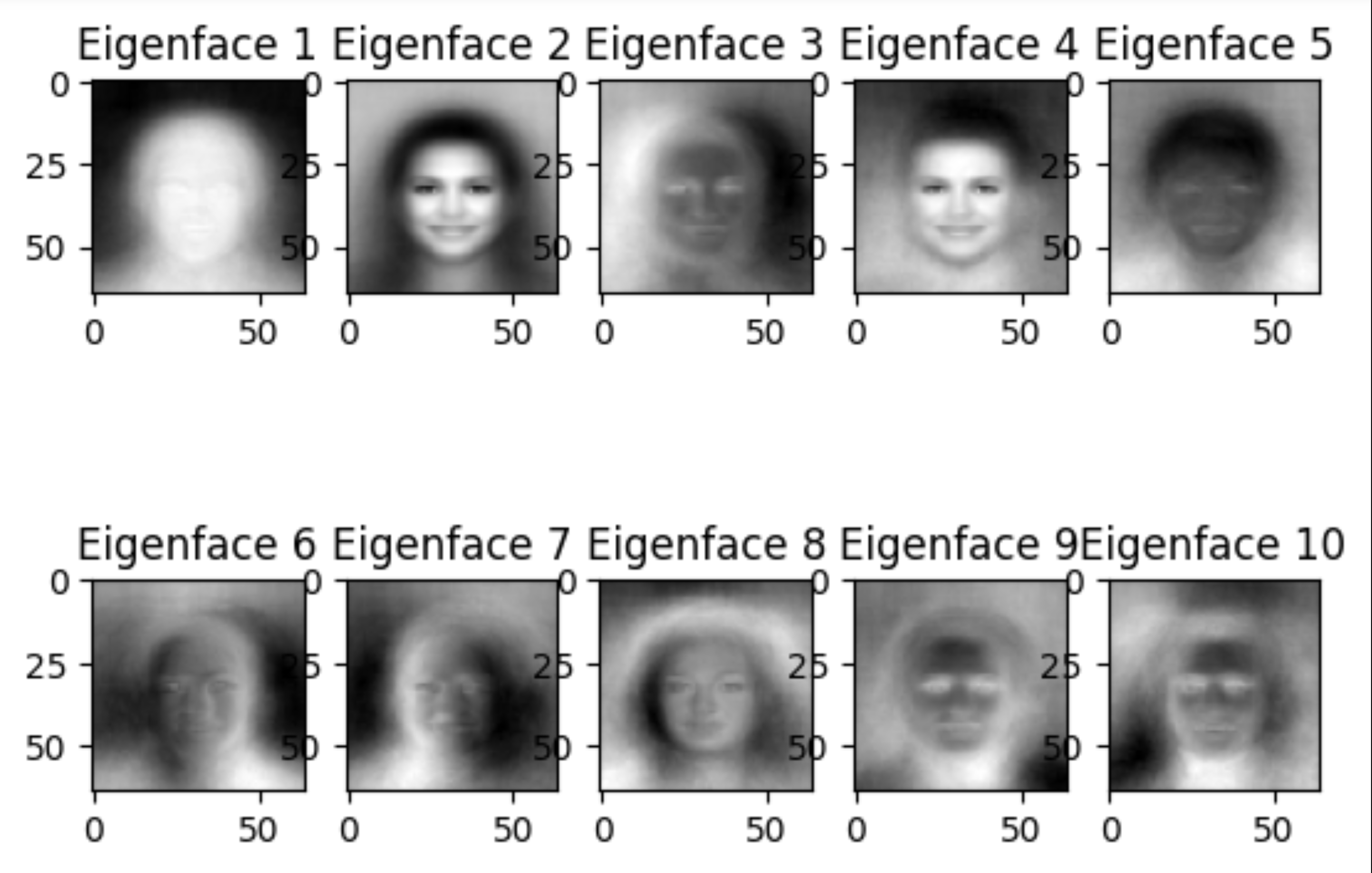
Why do some rows look like faces? Each row of $V^T$ is a direction in image-space, and $\sigma_i$ says how much variance the data has along it. The top rows grab the most global patterns in the dataset, and since the dataset is faces, those patterns are faces. Further down the list, the singular values shrink and the rows pick up on smaller variations, then just noise.

Generating a Face

We can also run the decomposition backwards to make new faces. Pick some random coefficients, weight them by the singular values, and mix the top rows of $V^T$ together. Add the mean face back on and you’ve got a new face pulled from the same linear space as the dataset.

def generate_random_face(Vt, s, mean_face, r=100):
  c = np.random.randn(r) * s[:r]
  face = mean_face + c @ Vt[:r]
  face = np.clip(face, 0, 255)
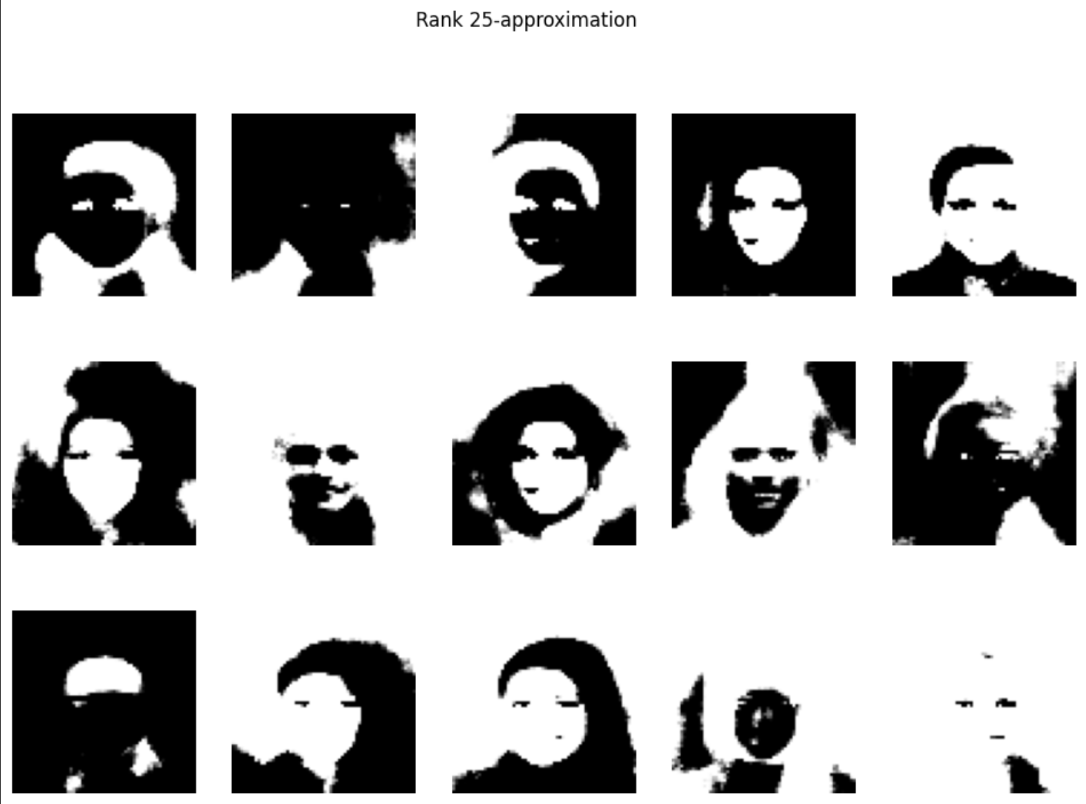
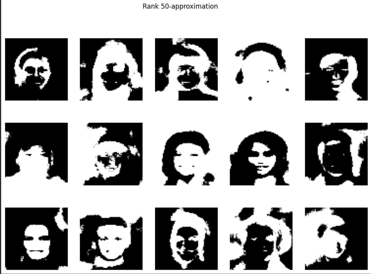
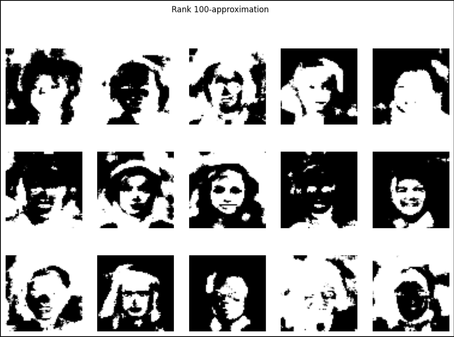
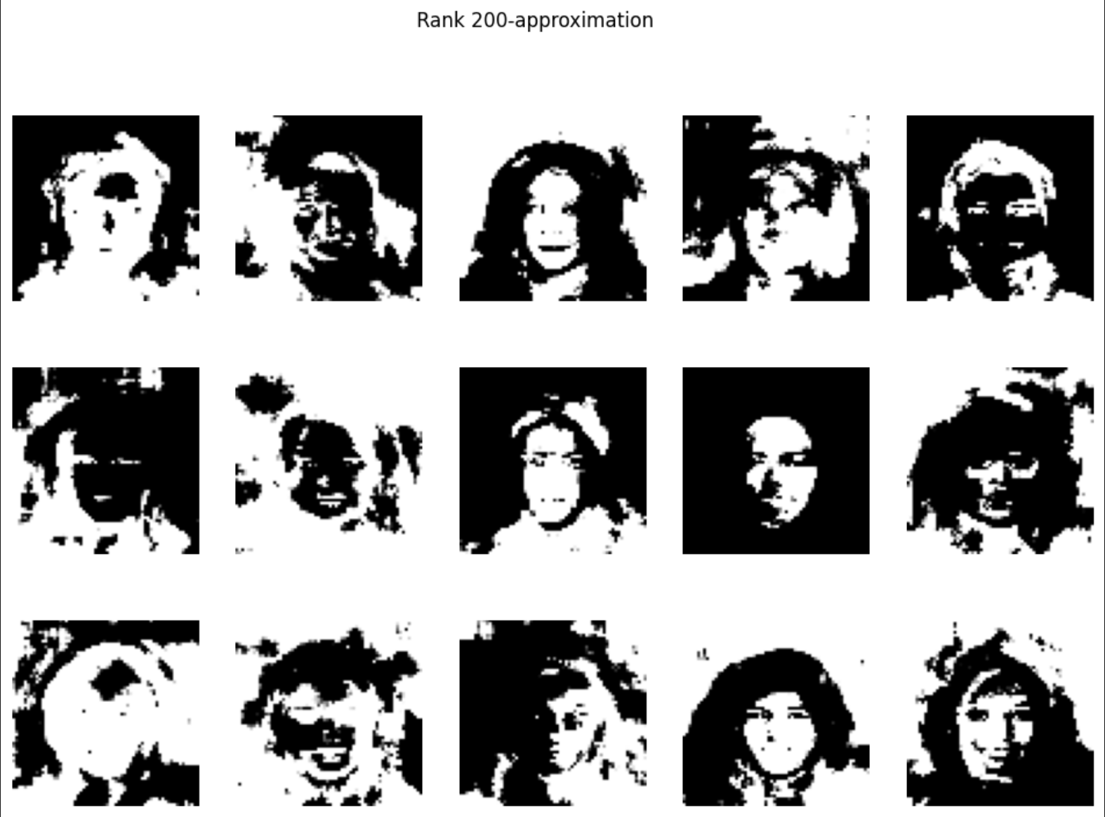
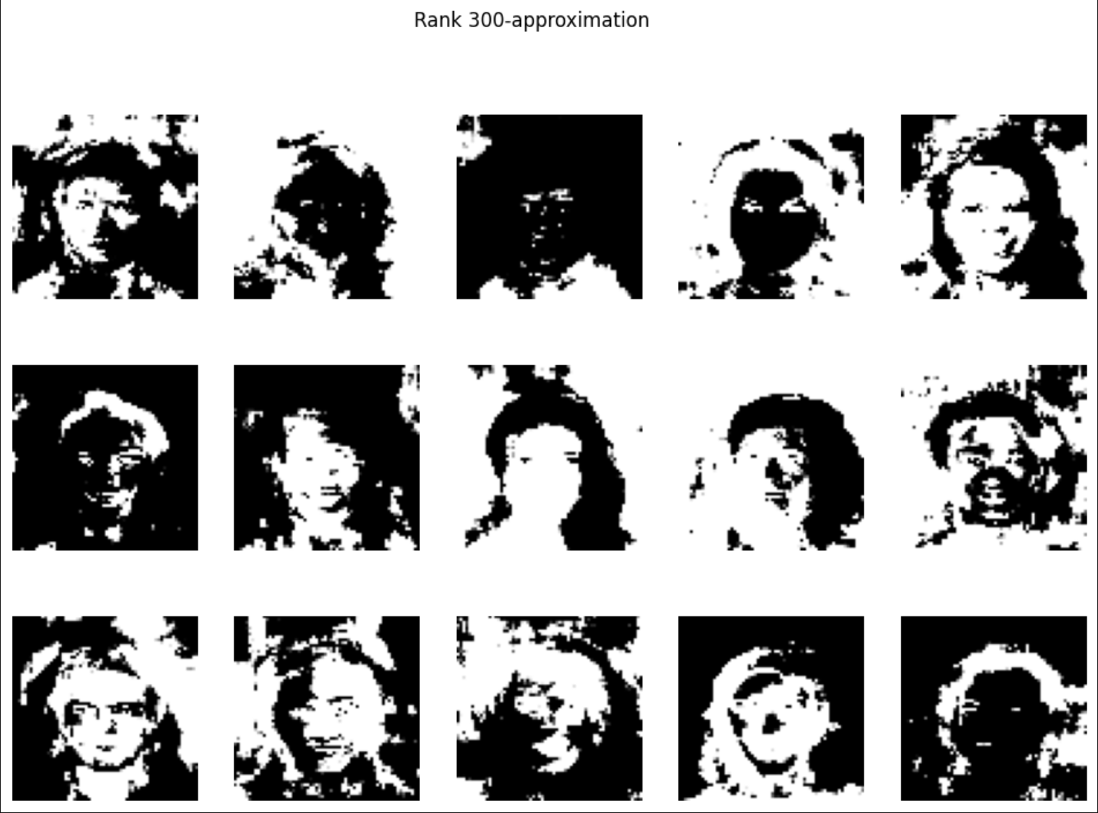
  return face.reshape(64, 64)

$r$ is the rank of the approximation. Like we saw earlier, the top rows of $V^T$ carry the global structure and the tail is mostly noise, so a small $r$ keeps the big facial features and drops the rest. Here are some that I generated:

Another way…?

SVD gave us faces, but they’re globally blended — every eigenface is a ghostly mix of the whole dataset. We can do better.

Non-Negative Matrix Factorization (NNMF) is another way to break apart the image matrix. It factors $V \approx W H$ with the constraint that both $W$ and $H$ only have non-negative entries. That constraint is the whole point. With no subtraction allowed, the decomposition can’t build a face by cancelling features against each other, so it has to find additive parts instead of blends. In practice, the rows of $H$ come out looking like localized facial features (eyes, noses, hairlines) rather than full-face ghosts.

You can read more about Non-Negative Matrix Factorization here.

def NNMF(V, k=100, MAX_ITERATION=500):
  eps = 1e-9
  tol = 1e-4

  m, n = V.shape
  W = np.random.rand(m, k)
  H = np.random.rand(k, n)
  previous_error = np.inf

  for i in range(MAX_ITERATION):
    H_num = W.T @ V
    H_den = W.T @ W @ H + eps
    H *= (H_num / H_den)

    W_num = V @ H.T
    W_den = W @ H @ H.T + eps
    W *= (W_num / W_den)

    current_error = np.linalg.norm(V - W @ H, 'fro')
    diff = abs(previous_error - current_error)

    if i > 0 and diff / previous_error < tol:
      break

    previous_error = np.linalg.norm(V - W @ H, 'fro')
  return W, H

Each loop applies the multiplicative update rules from the Wiki page to push $\|V - WH\|_F$ down. We bail out early once the error stops changing much.

Errors

We still have to pick good values for $k$ (the number of components) and MAX_ITERATION. To do that, we’ll sweep over a range of $k$ values and plot the reconstruction error.

errors = {}
error_ranges = list(range(1, 100, 10)) \
                + list(range(100, 200, 25)) \
                + list(range(200, 400, 75))  \
                + list(range(400, 500, 100)) \
                + list(range(500, 1000, 200))
# same as
error_ranges = [1, 11, 21, 31, 41, 51, 61, 71,
                81, 91, 100, 125, 150, 175, 200,
                275, 350, 400, 500, 700, 900]

That’s just the list of $k$ values we’ll try. Denser at the low end where the curve changes fast, sparser at the tail. Tweak it however you want.

For each $k$ we compute the reconstruction error $\|V - WH\|_F$. We also track its discrete derivative $d(\text{error})/dk$ so we can spot the elbow.

errors = {}
error_ranges = list(range(1, 100, 10)) \
                + list(range(100, 200, 25)) \
                + list(range(200, 400, 75))  \
                + list(range(400, 500, 100)) \
                + list(range(500, 1000, 200))
error_ranges = sorted(set(error_ranges))

for k in tqdm.tqdm(error_ranges):
    W, H = NNMF(images, k, 100)
    WH = W @ H
    errors[k] = np.linalg.norm(images - WH, 'fro')

keys = list(errors.keys())
vals = list(errors.values())

d_errs = {
    keys[i]: (errors[keys[i]] - errors[keys[i-1]]) / (keys[i] - keys[i-1])
    for i in range(1, len(keys))
}

fig, (ax1, ax2) = plt.subplots(1, 2, figsize=(14, 5))

ax1.plot(keys, vals)
ax1.set_title("Reconstruction Error")
ax1.set_xlabel("k")
ax1.set_ylabel("Frobenius Norm")

ax2.plot(list(d_errs.keys()), list(d_errs.values()))
ax2.set_title("d(Error)/dk")
ax2.set_xlabel("k")
ax2.set_ylabel("Error Rate of Change")

plt.tight_layout()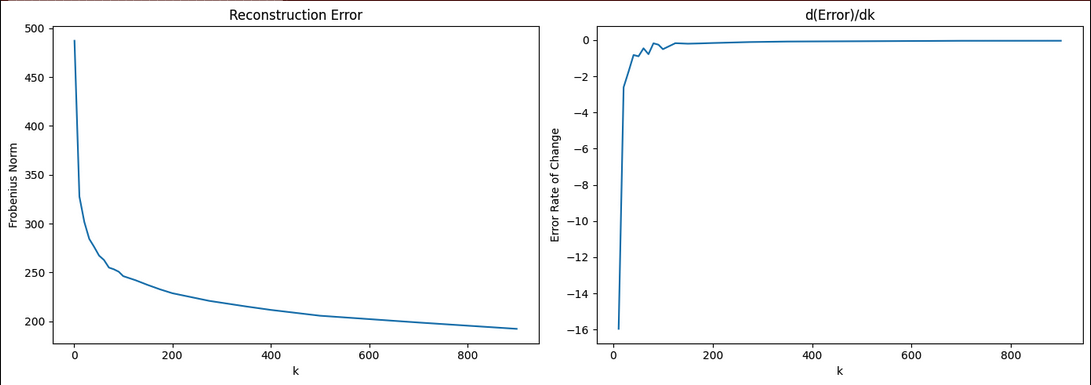

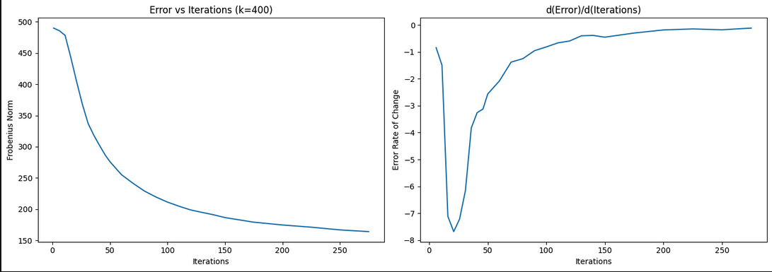
The error curve flattens out and $d(\text{error})/dk$ settles near zero around $k \approx 200$, so we’ll go with $k = 200$ and MAX_ITERATION $= 200$.

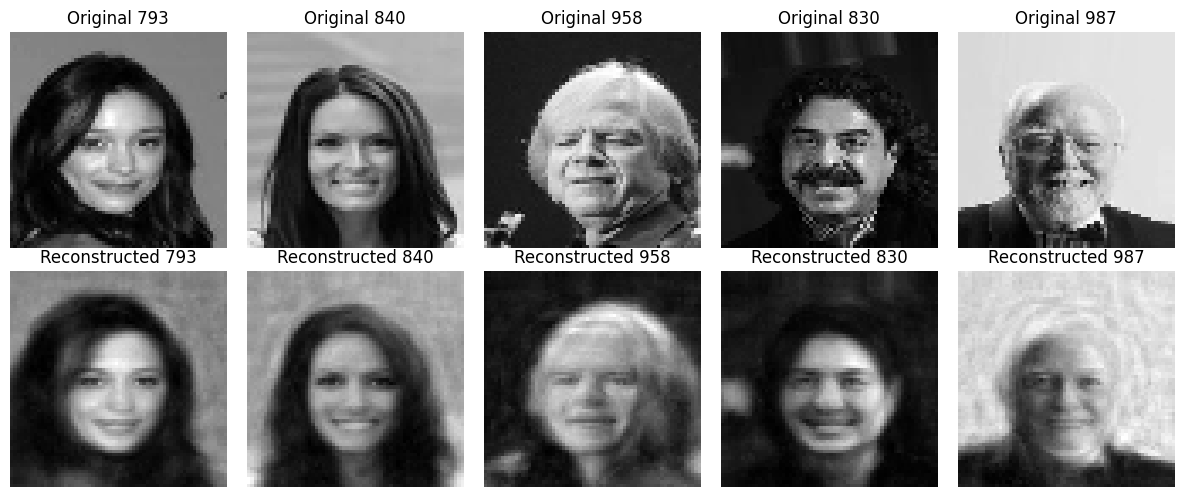
Now let’s reconstruct some faces and see how the model does.

Reconstruction!

Running this plots each original next to what the model reconstructs from $W$ and $H$.

W, H = NNMF(images, 200, 200)
def reconstruct_face(idx):
    # W[idx] is the coefficient vector for image idx, shape (k,)
    # W[idx] @ H is a weighted sum of the k components
    reconstructed = W[idx] @ H  # shape (n,) = (4096,)
    return reconstructed.reshape(64, 64)

# Plot original vs reconstructed
fig, axes = plt.subplots(2, 5, figsize=(12, 5))
counter = 0
amount = 5
pictures = random.choices(list(range(0, images.shape[0])), k = amount)
for i in pictures:
    original = images[i].reshape(64, 64)
    reconstructed = reconstruct_face(i)

    # Normalize for display
    reconstructed = np.clip(reconstructed, 0, 255)

    axes[0, counter].imshow(original, cmap='gray')
    axes[0, counter].set_title(f'Original {i}')
    axes[0, counter].axis('off')

    axes[1, counter].imshow(reconstructed, cmap='gray')
    axes[1, counter].set_title(f'Reconstructed {i}')
    axes[1, counter].axis('off')
    counter += 1

plt.tight_layout()

We can also use NNMF as a compression scheme. Instead of storing a full 64×64 image per face, we only need that face’s coefficient vector $W_i$ (length $k$), plus one shared $H$ for the whole dataset.

per_image_original = images[0].nbytes
per_image_compressed_amortized = W[0].nbytes + H.nbytes / len(images)
ratio = per_image_compressed_amortized / per_image_original
print(f"Compressed size is {ratio:.4f}x the original")

Which gives me the output:

Compressed size is 0.4977x the original

Roughly half the size. Sick!

We can also look at the features themselves to see what the model learned:

fig_row_count = 3
fig_col_count = 4

feature_importance = W.sum(axis=0)
top_indices = np.argsort(feature_importance)[::-1][:fig_row_count * fig_col_count]

# Auto-scale figure height based on grid size
fig, axes = plt.subplots(fig_row_count, fig_col_count, figsize=(10, 10))

for i, ax in enumerate(axes.flat):
    component = H[top_indices[i]]
    component = np.clip((component - component.min()) / (component.max() - component.min() + 1e-9), 0, 1)
    component = component.reshape(64, 64)
    axes[i // fig_col_count, i % fig_col_count].imshow(component, cmap='gray')
    axes[i // fig_col_count, i % fig_col_count].set_title(f"Feature {top_indices[i]}", fontsize=16)
    # ax.axis('off')

plt.tight_layout()
plt.show()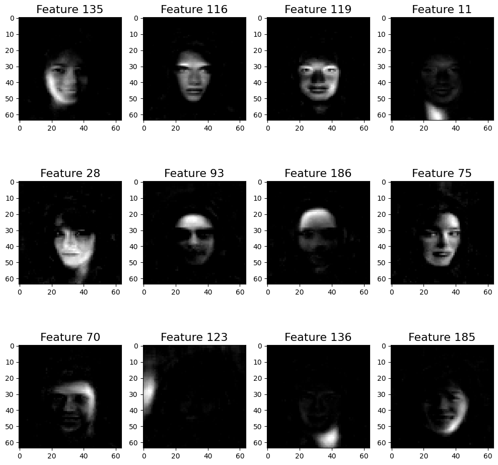

Alright, last step, just for fun: let’s sample some random faces from the NNMF model, same as we did with SVD. Since every coefficient in $W$ has to be non-negative, we sample from a Gaussian fit to each column of $W$ and clip any negatives back to zero.

def generate_random_face(mean, std, H):
    coeffs = np.clip(np.random.normal(mean, std), 0, None)
    face = coeffs @ H
    return np.clip(face, 0, 255).reshape(64, 64)

mean = W.mean(axis=0)
std  = W.std(axis=0)

fig, axes = plt.subplots(4, 5, figsize=(12, 10))
for ax in axes.flat:
    ax.imshow(generate_random_face(mean, std, H), cmap='gray')
    ax.axis('off')
plt.tight_layout()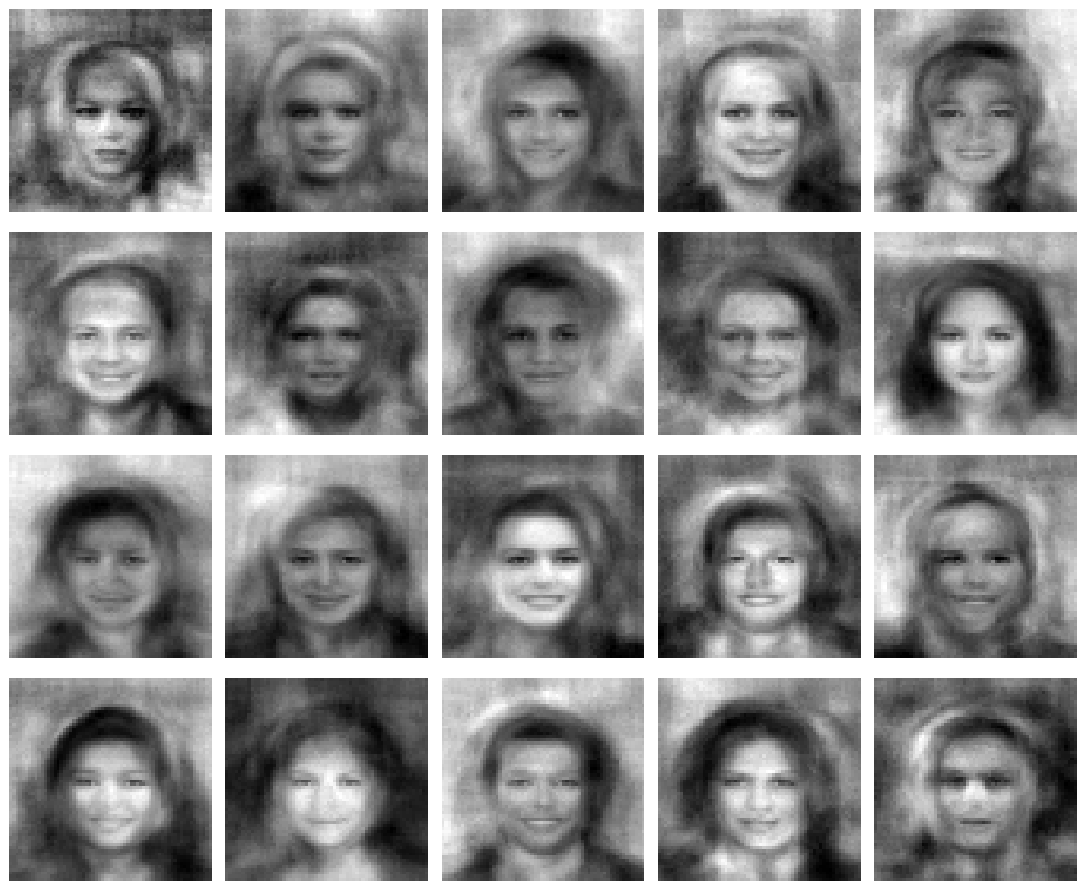

Compared to the SVD samples, these have way sharper facial features. The non-negativity constraint is doing exactly what we wanted: pushing the model toward parts instead of blends.